Microsoft Excel Functions Practice VLookup and HLookup

 VLOOKUP

VLOOKUP is probably the most popular function in Excel, and one of the most helpful functions for everyday use.

VLOOKUP helps us lookup a value in table, and return a corresponding value.

A good example for VLOOKUP in real life is our “Contacts” app on the phone:

We lookup for a friend’s name, and the app returns its number. This is exactly what VLOOKUP does!

Syntax

=VLOOKUP(lookup_value,table_array,col_index_num,[range_lookup]

• lookup_value – what we are looking for – this could be a text, number, or a single cell reference
• table_array – the range in which we will lookup for our value and its corresponding result. Please note that the range must start from the column which contains the value, and should contain the column in which we have our result.
• col_index_num – What is the column number from which we want to return the result? The number should be relative to the first column in the selected range in table_array.
• [range_lookup] – Which range lookup method should be used. 0 is the default, so you should always type 0 (or FALSE), which means “Exact Match” – Go to the exact match to the value I’m looking for. 1 stands for “Approximate match”, and it should not be used on most cases so we’ll skip it for now.

Here’s a quick example – let’s try to find out the age of the person with ID number #646:

• lookup_value –  we typed 646. We could as well reference a cell containing the number 646.
• table_array – This is where we perform our lookup. Our table starts at column B, as this is the column which contains our ID number. We can see that our table contains the Age column as well, as we would like to return the Age from it.
• col_index_num – we typed 2, as column C’s relative position is 2, if we consider that our table starts at column B.
• [range_lookup] – We are looking for an exact match, hence we type 0.

So what happens here is that the function goes to the table in range B1:C5, looks up in column B for the value 646, goes to the 2nd column in that table (Column C), and returns the corresponding value from it – 72.

Please note that if we tried to return the Name column instead of Age column, we would not be able to do so with VLOOKUP unless we changed the position of columns. The reason for that is because column A is before Column B, which must be the first column in table_array as it contains the ID number. In such case, it is recommended to use INDEX MATCH instead, or even better – use the almighty XLOOKUP function.

HLOOKUP

Explanation

HLOOKUP  is a powerful Excel function used to search for a value in a table or a range by matching it with data in a row. HLOOKUP is very similar to very popular function called VLOOKUP –  While VLOOKUP searches vertically in columns, HLOOKUP searches horizontally in rows. 

HLOOKUP is useful when the data is organized horizontally, with the lookup values in the first row and the corresponding data in rows below. 

Syntax 

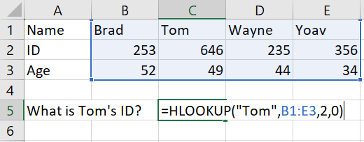
=HLOOKUP(lookup_value, table_array, row_index_num, [range_lookup]) 

• lookup_value – The value you are searching for, which can be text, number, or a cell reference.
• table_array – The range where you will perform the lookup. The range must start with the row containing the lookup value and should include the row from which you want to return the result.
• row_index_num – The row number from which you want to return the result. The number should be relative to the first row in the selected range in table_array.
• [range_lookup] – Which range lookup method should be used. In most cases we are using exact match and therefore if this is your first time using the function –  we recommend using 0 (zero) or FALSE, both are for “Exact Match” – Go to the exact match to the value I’m looking for. 1 stands for “Approximate match”, and it should not be used on most cases so we’ll skip it for now.

Example 

Here’s a quick example – let’s try to find out the age of the person with ID number

Please note that if we tried to return the Name row instead of Age row, we would not be able to do so with HLOOKUP unless we changed the position of rows. The reason for that is because row 1 is before row 2, which must be the first row in table_array as it contains the ID number. In such case, it is recommended to use INDEX MATCH instead, or even better – use the versatile XLOOKUP function. 

Practice HLOOKUP